Fedea - Lost in Recession: Youth Employment and Earnings in Spain
←
→
Transcripción del contenido de la página
Si su navegador no muestra la página correctamente, lea el contenido de la página a continuación
Estudios sobre la Economía Española - 2021/12

Lost in Recession: Youth Employment and Earnings in Spain

                              Samuel Bentolila
                                 (CEMFI)

                           Florentino Felgueroso
                                  (Fedea)

                              Marcel Jansen
                              (UAM y Fedea)

                             Juan F. Jimeno
                (Banco de España y Universidad de Álcala)

                                 Marzo 2021

                                 fedea

       Las opiniones recogidas en este documento son las de sus autores
              y no coinciden necesariamente con las de FEDEA.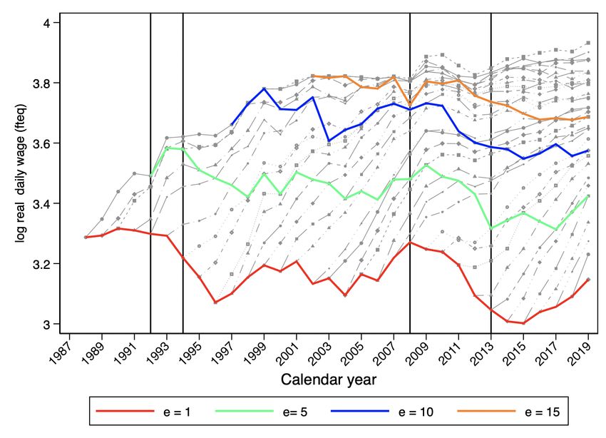
Resumen

La actual generación de jóvenes se enfrenta a retos excepcionales, tras sufrir el impacto de
dos crisis económicas profundas en poco más de una década. En el caso de España este reto
es aún mayor debido a problemas estructurales en el mercado de trabajo que perjudican
especialmente a los jóvenes, dificultando su acceso a empleos estables. Motivado por estos
hechos, el presente estudio analiza la evolución de las condiciones laborales de los jóvenes
durante los últimos treinta años y documenta su continuo deterioro. En cada recesión se
produce un retroceso en la situación laboral de los jóvenes. Los principales afectados son
quienes terminan sus estudios durante estas recesiones, que sufren impactos negativos sobre
su empleo y sus salarios no solo al entrar en el mercado de trabajo sino también durante un
buen número de años de su carrera profesional. En otras palabras, les quedan cicatrices, por
lo que este fenómeno se conoce como el “efecto cicatriz de las recesiones”. Sin embargo, el
principal resultado de este estudio es la falta de una recuperación completa de las condiciones
laborales que tienen los jóvenes al inicio de una recesión durante la siguiente expansión, en
particular, los días medios trabajados y los ingresos laborales correspondientes. Es decir, que
una parte considerable del deterioro sufrido en las recesiones se consolida, provocando una
tendencia negativa en las condiciones iniciales de empleo de cada cohorte siguiente de
jóvenes en España.

El estudio se divide en tres partes. La primera parte ofrece una panorámica de las principales
tendencias del mercado de trabajo de los jóvenes usando datos procedentes de la Encuesta de
Población Activa (EPA) y la Muestra Continua de Vidas Laborales (MVCL). Esta segunda
fuente incluye el historial laboral de una muestra representativa del 4% de los cotizantes a la
Seguridad Social. Aparte de hechos ya conocidos, como la alta volatilidad cíclica del paro
juvenil y la alta proporción de contratos temporales, los datos muestran la delicada situación
de los jóvenes al principio de la actual pandemia, con tasas de paro que duplican las
existentes al principio de la Gran Recesión de 2008-2013. Sin embargo, el hecho más
destacable es la senda negativa de los ingresos salariales de los jóvenes. En 2019, la mediana
del salario mensual real de los jóvenes entre 18 y 35 años era menor que en 1980, con caídas
que van desde el 26% para aquellos con edades entre 30 y 34 años hasta el 50% para los de
18 a 20 años. Estas caídas se deben principalmente a una reducción muy acusada de la
duración de sus empleos y a un aumento del peso del empleo a tiempo parcial. El impacto
conjunto supone caídas de la media de los días de trabajo equivalentes a tiempo completo del
73% al 22%, respectivamente, debido a la caída de la duración de los contratos y de la
jornada laboral.

Para entender mejor estas tendencias, en la segunda parte se presenta un análisis al nivel de
las cohortes empleando datos longitudinales de la MCVL. Al igual que la mayoría de los
estudios sobre los efectos cicatriz de las recesiones, este análisis se limita a los jóvenes con
estudios universitarios a los que se divide en función de su titulación: diplomatura, grado y
posgrado. Los principales resultados confirman las tendencias identificadas en la primera
parte. En particular, durante las recesiones se observa una fuerte caída de la renta laboral
media de los jóvenes durante su primer año en el mercado de trabajo. Además, las cohortes
que entran en los años posteriores a cada recesión lo hacen en condiciones similares o incluso
peores. El resultado es una caída tendencial en la renta salarial durante el primer año de
experiencia laboral y lo más llamativo es que se producen patrones similares, aunque menos
acusados, hasta los 15 años de experiencia laboral, lo que sugiere que el deterioro de las
condiciones de entrada tiene efectos persistentes durante buena parte de las carreras laborales.

En la tercera y última parte se lleva a cabo un intento de medir la persistencia de las
condiciones de entrada en el mercado. En el análisis empírico se utiliza la variación al nivel
de la cohorte de la tasa de paro provincial y del año de graduación, para estimar en qué
medida condiciones desfavorables en el momento de la entrada al mercado de trabajo
condicionan el progreso de los resultados laborales en los años posteriores. Este análisis es
estándar en la literatura sobre el efecto cicatriz de las recesiones. Sin embargo, una de las
novedades de este estudio es que también se permite que exista una senda temporal diferente
para cada nivel de experiencia laboral (interactuando una tendencia con “efectos fijos” de
experiencia potencial). Esto permite captar el impacto de cambios estructurales en el mercado
de trabajo –que pueden ser cambios de la oferta o la demanda de universitarios o de los
aspectos institucionales– sobre los resultados laborales de los jóvenes durante sus primeros
diez años en el mercado.

Los resultados obtenidos confirman la importancia de las condiciones iniciales. En la
especificación de referencia para quienes terminan un grado universitario, una subida de un
punto porcentual de la tasa de paro provincial en el año de entrada está asociada con una
caída de la renta salarial mensual de 1,5 puntos porcentuales dos años después. Y el efecto
solo deja de ser significativo a partir del séptimo año. A modo de ejemplo, estas cifras
implican que el universitario medio graduado en 2013 en la provincia con la menor tasa de
paro en 2007 (Guipúzcoa) obtendría dos años más tarde una renta mensual un 13,5% más
baja que la de alguien que hubiera entrado en 2007, mientras que la pérdida correspondiente a
la provincia con la mayor tasa de desempleo (Jaén) hubiera sido cercana al 40%. No obstante,
estos efectos estimados son algo menores que en la mayoría de los estudios existentes y
desaparecen casi completamente al introducir como factores explicativos los cambios
estructurales (la senda temporal antes mencionada), niveles medios distintos para cada
cohorte y la tasa de paro nacional contemporánea. Por el contrario, los efectos de la senda
temporal para cada nivel de experiencia son grandes y estadísticamente significativos. En
concreto, comparando a dos individuos que se gradúan con diez años de diferencia en la
misma provincia y con la misma tasa de paro provincial, el salario diario medio y el número
de días trabajados durante el primer año serían respectivamente un 7% y un 9,3% más bajos
para la persona que entra más tarde. Por tanto, al considerar un período de tiempo
suficientemente largo, pesa más el año de entrada al mercado de trabajo que la tasa de paro en
el momento de la graduación.

Se deja para la investigación futura el estudio de las causas del continuo deterioro de las
condiciones laborales iniciales de los jóvenes. Una posible causa es la introducción de
reformas laborales durante las recesiones que flexibilizan la contratación y/o el despido de los
jóvenes y que acaban precarizando aún más su empleo. Sin embargo, tampoco hay que
descartar la importancia de los desajustes entre la oferta y la demanda de cualificaciones
debido al progreso tecnológico y el poco peso de las disciplinas STEM (ciencia, tecnología,
ingeniería y matemáticas) en nuestro país.
Lost in Recession: Youth Employment and Earnings in Spain*

                                            Samuel Bentolila
                                               CEMFI

                                         Florentino Felgueroso
                                                 Fedea

                                          Marcel Jansen
                                 Universidad Autónoma de Madrid

                                        Juan F. Jimeno
                           Banco de España and Universidad de Alcalá

                                             22 March 2021

                                                 Abstract

Young workers in Spain face the unprecedented impact of the Great Recession and the
Covid-19 crisis in short sequence. Moreover, they have also experienced a deterioration
in their employment and earnings over the last three decades. In this paper we document
this evolution and adopt a longitudinal approach to show that employment and earnings
losses suffered by young workers during recessions are not made up in the subsequent
expansions. We also estimate the size of the scarring effects of entering the job market in
a recession for college-educated workers during their first decade in the labor market. Our
empirical estimates indicate that, while there is some evidence of scarring effects, the
driving force is a trend worsening of youth labor market outcomes.

Key words: youth, employment, earnings, scarring effects.
JEL codes: J13, J24, J31.

*
 Bentolila is also affiliated with CEPR and CESifo, Jansen with Fedea and IZA, and Jimeno with CEPR
and IZA. Bentolila acknowledges financial support from the Spanish Ministry of Science and Innovation
under grant PID2019-111694GB-I00 and Jansen under grant PID2019-107916GB-100. The views
presented here are solely of the authors and not of any of the institutions to which they are affiliated with.

                                                      1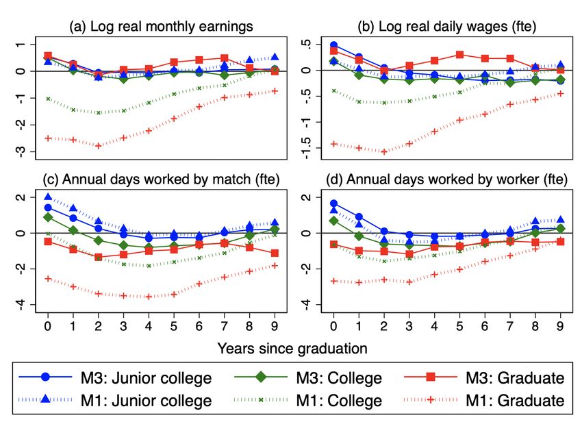
1. Introduction

Spanish youth face a tremendous challenge. Their welfare was severely hit by the Great
Recession (2008-2013) and they are now battered by the recession caused by the Covid-
19 pandemic that started in 2020, which is beating them especially hard. This is a matter
of the utmost importance for the Spanish society.

Moreover, this is not a new situation. The Spanish labor market is a hostile environment
for young workers. “No country for young people”, in the apt expression of Juan J.
Dolado, a great economist, a close friend of ours, and a movie buff. A couple of figures
make this evident. Over the period 1983-2019, the average unemployment rate for
workers aged 20-24 years old was equal to 32.7% and for those aged 25-29 years old it
was equal to 22.3%. In contrast, in the (then) European Union of 28 countries (EU-28),
the corresponding averages were, respectively, 17.8% and 11.5%, in other words, about
half the size of the rates in Spain.

And this is not simply the result of the overall unemployment rate being significantly
higher in Spain than in the rest of Europe. Young Spaniards suffer on every front: they
have very low employment rates, very high rates of temporary employment with a
corresponding huge job churn, and low wages.

The economic analysis of the causes of low employment rates and high unemployment
rates among young workers can be divided into two strands of research. The first one
studies the relevance of education, labor market institutions, and employment policies on
the transition from school to work to the determination of structural unemployment. A
second strand of research analyzes the cyclical behavior of youth unemployment and the
scarring effects of entering the labor market during recessions.

In line with this dichotomy, the problems for young workers’ transition from school to
work in Spain are found on two fronts. The first one is education, with key aspects like
the levels of attainment, the composition by disciplines or its quality. In this regard, Spain
suffers from a high dropout rate –which was especially high during the expansion that
preceded the Great Recession– and at the same time a relatively high share of university
graduates (mostly in Law, Humanities, and Social Sciences) and a low share of upper
secondary education, mostly due to a shortfall in vocational education and training. The
second front is related to labor market institutions, which strongly worsen the
employment opportunities of new entrants. With an entrenched dual configuration,
employment protection legislation and the structure of collective bargaining create a
strong insider-outsider divide that place a significant burden on youths (Bentolila et al.
2012, 2020, Felgueroso et al. 2019).

Beyond the structural causes of youth unemployment and the long-run trends affecting
this segment of the labor market –i.e., demographics, technology, and human capital
accumulation– the current cohorts of young workers have been very negatively affected
by two deep recessions taking place in short sequence. Indeed, the economic impacts of
both the Great Recession and the Covid-19 crisis have been particularly acute in
comparison with the rest of Europe. The former was associated with the bursting of a
housing bubble and the subsequent downsizing of the construction sector –where many
school dropouts were employed– and the latter has strongly reduced employment
opportunities in the service sector –in which job entry ports for young people were

                                              2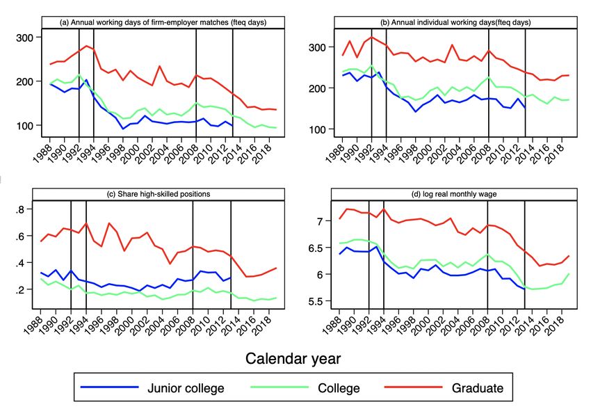
overrepresented. Thus, we should expect the scars from entering the labor market in a
recession to be deeper for the current cohorts of young Spaniards than for their European
counterparts.

There is a small but growing literature on the scarring effects of recessions. Most studies
focus on university graduates and base their empirical strategy on the seminal
contribution of Oreopolous et al. (2012) for the case of Canada. This study exploits the
variation across cohorts and provinces in the unemployment rate to study how the labor
market conditions at graduation condition entrants’ experience profiles of earnings and
employment. In the case of the US there are several studies that point at substantial
scarring effects using a similar setup (e.g., Kahn 2010, Altonji et al. 2016, Schwandt and
von Wachter 2019 or Rothstein 2020). According to these studies a deep recession causes
a drop in initial earnings of close to 10%, with estimated semi-elasticities of earnings with
respect to the unemployment rate in a range between 2 and 3. The negative effects remain
significant up to seven years after entry. In most studies, the drop in initial earnings is
attributed above all to a fall in the number of days of work along with a drop in the quality
of the entrants’ first job. Indeed, mobility to other jobs is a key mechanism behind the
gradual recovery of earnings, especially in the first years after entry. By contrast, in later
years, convergence in earnings mainly takes place through wage growth at the same
employer. Furthermore, the studies for the US and Canada point at substantial variety in
the strength of the scarring effects by field of study, college attended, and type of
program. In general, the scarring effects are weaker and less persistent for individuals
with the highest predicted level of future earnings. Besides earnings and employment,
recent studies have also considered outcome variables such as household income, access
to welfare payments or poverty. Finally, two studies (Altonji et al. 2016 and Rothstein
2020) document much larger losses for individuals who entered the US labor market
during or after the Great Recession. Altonji et al. (2016) attribute this trend break, which
both studies date around 2005, to a rise in the cyclical sensitivity of the employment of
college graduates.

Apart from Canada and the US, evidence on the scarring effects of recessions is available
for a range of countries.1 As for Spain, Fernández-Kranz and Rodríguez-Planas (2017)
use Social Security records that cover the period 1980-2008 to analyze the scarring effects
from recessions for males at all levels of education, using a setup based on Kahn (2010).
In this simplified setup, the initial unemployment rate is interacted with a continuous
variable that measures entrants’ potential experience rather than cohort fixed effects as in
Oreopolous et al. (2012). According to their findings, the negative effects from entry in
recessions fall with the educational attainment of entrants. In particular, for high school
graduates they obtain initial earnings losses in deep recessions of 25%, that drop to 3%
after 10 years. By contrast, for university graduates the initial impact is half as big and
the penalty ceases to be significant after five years.

Our paper offers various contributions to the analysis of youth employment and earnings
of young Spaniards. First of all, our sample period spans the period 1987-2019. Hence,
our estimation includes the cohorts that entered during the Great Recession. Furthermore,
while our empirical strategy is closer to the one developed by Oreopoulos et al. (2012),
we pay more attention to the relative relevance of both the initial labor market conditions

1
 The list of countries includes Australia (Andrews et al. 2020), Austria (Brunner and Kuhn 2014), Belgium
(Cockx and Girelli 2015), Germany (Arellano-Bover 2020), Japan (Genda, Kondo, and Ohta 2010) and
Norway (Raaum and Roed 2006).

                                                   3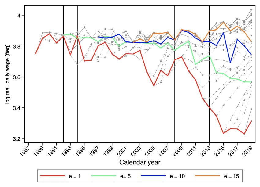
at graduation and the actual year of entry. This issue is key because inspection of the data
reveals a clear negative trend in the initial labor market outcomes of university graduates
in Spain. To be more precise, in recessions we observe a steep deterioration in the initial
outcomes of graduates, but in the subsequent recovery the initial conditions for later
cohorts do not recover their pre-recession levels. In other words, a substantial share of the
deterioration in labor market outcomes of graduates in recessions is consolidated, causing
a trend decline in the initial conditions of university graduates.

The rest of this paper is organized as follows. We start by documenting in Section 2 the
trend deterioration experienced in the labor market for youths in Spain over the last three
decades, focusing on aggregate youth unemployment and employment rates, and
temporary and part-time employment rates; and discuss developments in education and
in the days worked and earnings of young workers. Then in Section 3 we adopt a cohort
approach and show, over the same period, the longitudinal evolution of employment and
earnings of young workers from job market entry onwards, finding that losses suffered
during recessions are not made up in the subsequent expansion. In Section 4 we estimate
the size of scarring effects. We trace how the state of the labor market at the graduation
dates affects the employment and earnings of young workers during their first decade in
the labor market. We find that, while there is some evidence of scarring effects, the
overriding force appears to be a trend worsening of youth labor market outcomes. In
Section 5 we summarize the conclusions from our analysis.

2. The Spanish youth labor market: An overview

There are well-known reasons why young workers suffer higher unemployment rates and
earn lower wages than adult workers. Young workers are more mobile, have lower job
experience, and, after transiting from school to work, are more likely to enter into job
matches that are of lower duration and less adequate to their professional skills. Typically,
as working life proceeds, workers settle down into significant and stable jobs, where
experience, earnings, and job stability improve, resulting in better labor market outcomes.

However, even after taking these factors into account, the Spanish labor market for youths
shows a dismal performance.2 Three facts are striking. The first one is that differences
between the labor market outcomes of young and adult workers are huge in comparison
to most European countries. The second one is that over the last four decades, the labor
market outcomes of Spanish youths have significantly worsened. Lastly, the speed at
which young workers enter into more stable and rewarding employment spells is
extremely low. What follows is a brief overview that documents these three facts.

To start our discussion, Figure 1 shows unemployment rates by age group in Spain and
the EU-28 from 1983 to 2020. During this period, unemployment rates in Spain fluctuated
around an average of 32.7% for the 20-24 year olds, 22.3% for the 25-29 year olds, and
13.1% for the 30-64 year olds.3 In contrast, in the EU-28 the corresponding averages
were, respectively, 17.8%, 11.5% and 7.1%. Thus, the gaps between young and adult
workers’ average unemployment rates in Spain almost double the ones observed in the
EU-28, e.g., 19.6 % in Spain vs. 10.7% for the 20-24 year olds vis-à-vis the 30-64 year

2
 For a comparison across European countries see Dolado (2015).
3
 We informally use an extended definition of youth, going up to 29 years old, as opposed to the standard
definition that stops at 24 years old.

                                                   4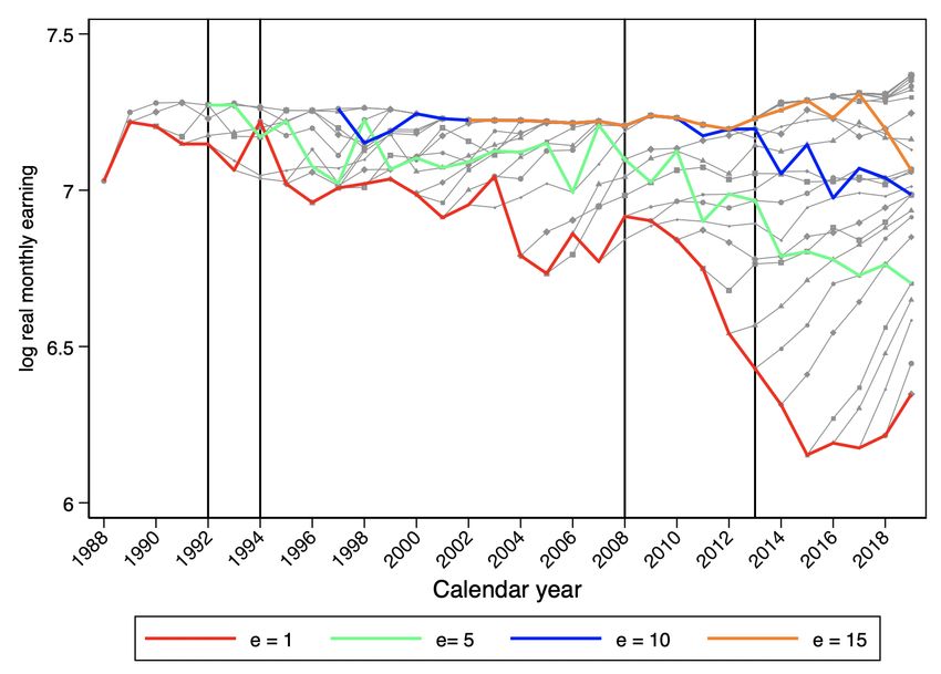
olds.4 It is also worth noting that the rises in unemployment rates in recessions (shaded
areas in the figure) are much more pronounced in Spain for young workers than for adult
workers, while in the EU-28 the unemployment rates for different age groups move more
or less in parallel. For instance, while the gap in unemployment rates of the 20-24 year
olds with respect to 30-64 year olds in 2007 was the same in the EU-28 and Spain, 8.2
percentage points (pp), by 2013 it had increased to 13.4 pp in the EU-28 and a whopping
29 pp in Spain.

As indicated, the second feature is that, despite the strong recovery following the Great
Recession, youths are now entering a new crisis with much higher unemployment rates:
in 2007 the youth unemployment rates for the 20-24 and 25-29 year-old groups were,
respectively, 15%, and 9%, while the corresponding rates in 2019 were, respectively,
29.8%, and 19%.

Fig. 1. Unemployment rates by age group, 1983-2020

Note: Annual data. Source: OECD Statistics (stats.oecd.org).

4
  For more information on international comparisons of unemployment fluctuations and some of their
determining factors, see Hernanz and Jimeno (2017).

                                                   5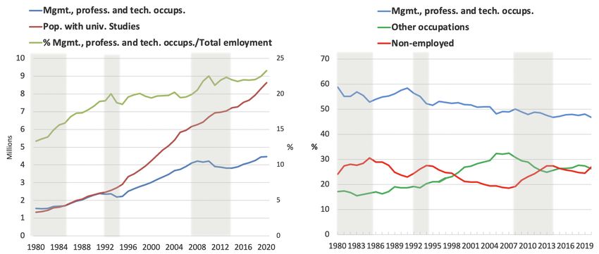
Lastly, the school-to-work transition is particularly slow in Spain. Data from the 2009 ad-
hoc module of the European Labor Force Survey (LFS) indicated that the average time
between leaving formal education and starting the first job for people with upper
secondary and post-secondary non-tertiary education was 7.3 months in the EU-27 vis-à-
vis 8.8 months in Spain. The figures for people with tertiary education were 5.1 and 7
months, respectively. More recent data indirectly reinforce the idea of a slow transition.
In 2019 the employment rate for people aged 15 to 34 years old in the EU-27 was equal
to 75.7%, while in Spain it was only 64.6%.

Figure 2 provides a more detailed account of the relative labor market performance of
young and adult workers in recent recessions. In the two recessions of the 1980s and early
1990s, young workers in the age group 25to 29 performed better than older age groups.
During this period the Spanish economy was undergoing a structural transformation, with
intense labor reshuffling from agriculture and traditional manufacturing to new
technology-intensive manufacturing industries and to services. At the same time,
university enrolment was strongly increasing. By contrast, all three recessions in the XXI
century are characterized by a clear monotonic age pattern with above-average reductions
in employment rate for young workers and below-average reductions or even a modest
increase in employment rates for prime age (30-54 years old) and older cohorts (over 55
years old).

Fig. 2: The fall in employment rates in recessions by age group, 1978-2020

Note: The figure shows the difference in log employment rates between the last quarter before the start of
a recession and the last quarter prior to the first increase in total employment. A recession is defined as two
consecutive quarters with negative GDP growth rate. For the first four recessions, net employment
decreases are depicted until the quarter prior to an increase in total employment. For the ongoing Covid-19
recession, we depict all the quarterly variations from 2019Q4 to 2020Q4. Dotted lines depict effective
employment excluding temporary layoffs. Sources: National Accounts GDP series and Labor Force Survey,
1976Q3-2020Q4, Instituto Nacional de Estadística (ine.es).

The higher impact of recessions on the employment rates of young workers is a general
phenomenon in most countries. Again, there are well-known reasons for this fact. Firms

                                                      6
typically use the LIFO principle (last-in, first-out) to adjust their labor force and
employment protection legislation tends to provide higher coverage to older workers
(with longer notice periods and higher severance payments for firing, among other
provisions). Thus, changes in job flows in recessions typically hit young workers harder.
When job creation falls, new entrants to the labor market are especially likely to find
fewer job opportunities and also poorer ones. When job destruction increases, those with
lower job experience and shorter employment spells are most likely to lose their jobs.
But, again, the magnitude of the differential in employment losses between young and
adult workers in Spain is peculiar and it cannot be separated from another characteristic
feature of the Spanish labor market: the prevalence of temporary contracts in new hires
(above 90% since the early 2000s).
Fig. 3: Total, temporary, and part-time employment rates by age group, 1988-2020
(a) Employment rate of youth not in education or (b) Temporary employment rates
training
(c) Part-time employment rates
Note: The three panels report backward-looking moving averages of four quarters. Source: Labor Force
Survey, Instituto Nacional de Estadística (ine.es).
Figure 3 provides information on the employment status of young workers. Panel (a)
shows that both the level and the stability of employment rates increase with age. On the
7other hand, the prevalence of temporary employment falls with age as shown in panel (b):
while the average temporary rate has fluctuated between 25% and 33% since the early
1990s (not shown in the figure), for young workers these rates hoover around 80%, 60%
and more than 40%, respectively, for the 18-20, 21-24, and 25-29 year-old groups. Even
for employees between 30 and 34 years old, the temporary rate is still around 30%, which
suggests that the transition between temporary and regular employment takes place at a
very low speed. Finally, panel (c) shows a marked increase in part-time employment since
2005, which, among other things, is relevant for the evolution of wages to be described
below.
Social Security data from the Continuous Sample of Working Lives (CSWL, see Data
Appendix) allow a closer examination of the early labor market outcomes of young
workers in Spain. For illustrative purposes, we use the 2019 wave of the CSWL to
compute annual statistics for earnings and days worked going back to the worker’s time
of labor market entry.5
Figure 4 plots the means of four variables: the annual days of work of individuals, the
annual days of work in a given firm-worker relationship, monthly earnings and full-time
equivalent daily wages of youths who worked at some point during the year (including
self-employment)6. For all four age groups we observe marked negative trends in annual
days worked, which are associated to both a reduction in the duration of temporary jobs
and the rise of part-time work shown in Figure 3. Panels (a) and (b) show that days worked
fall sharply in recessions and, surprisingly, barely stabilize in expansions, when job
opportunities increase across the board. Indeed, in 2019 our two indicators of the mean
days of work were still close to their all-time lows at the end of the Great Recession. As
for wages, panel (c) reveals a trend reduction of real monthly earnings, with strong losses
during recessions and partial recovery during expansions. When adjusted for working
hours, panel (d) shows the same initial fall, but then sustained rises for all groups
subsequently, which are weaker the older is the group of workers and still punctuated by
reductions during recessions.
5
Note that, due to this choice of sample, we are not reporting longitudinal variables, since individual
workers move up across lines as they age, and the data are affected by worker attrition.
6
Detailed descriptions of these variables appear in the next section and in the Data Appendix.
8Fig. 4: Annual days worked and wages by age group, 1980-2019
(a) Mean annual full-time equivalent (b) Mean annual full-time equivalent days worked
days worked in firm-worker relationships per worker
(c) Median log real monthly earnings (d) Median log real full-time equivalent daily wage
Notes: Panel (a): average length of employment relationships in a given calendar year, transformed into
full-time equivalent days of work using the part-time coefficient reported in the CSWL. Panel (b): same as
(a) for employees and the self-employed working in the corresponding year. Panel (c) Median monthly
earnings for employees in work. Panel (d) Median daily wage converted to full-time equivalent as in (a).
Source: Continuous Sample of Working Lives, Ministerio de Inclusión, Seguridad Social y Migraciones.
It is worth stressing that there are strong composition effects in the evolution of earnings
of young workers, since there has been a significant increase in their educational
attainment and, consequently, in the age of new entrants to the labor market. Figure 5
shows that dropout rates among youth decreased by around 45 pp during the last four
decades, while the proportion of university graduates among the young population is now
five times larger, in the case of women, and three times larger in the case of males, despite
the slowdown observed during the period of the housing bubble (2001-2008).
Consequently, the median age at transiting from school to work has risen by four years
for women and by three years for men since the late 1990s. This increase, partly
associated to reforms of university education, lowered the employment rates of the
9youngest workers even more, since simultaneously studying at university and working in
either seasonal or part-time jobs is very infrequent in Spain (less than 10% of the 18-24
year olds do it). Hence, most new entrants to the labor market have no previous labor
market experience. Moreover, as shown by Dolado et al. (2000) higher educated workers
crowd-out lower educated ones from their traditional entry jobs, so that a combination of
rigid labor market institutions and an increase in the relative supply of higher educated
workers harmed the training prospects of lower educated workers.
Fig. 5: Dropout rates, share of college graduates, and median age of completion of
the highest level of study, by gender, 1980-2019
(a) Share of early school leavers (18-24 y.o.) (b) Median age of completion of highest level of
and share of college graduates (25-29 y.o.) study
Notes: The data correspond to the native population. Source: Labor Force Survey, Instituto Nacional de
Estadística (ine.es).
Labor supply was not the only variable that changed during this period. The sectoral and
occupational structures of entry jobs for young workers went through a significant
reshuffle as well. Panel (a) in Figure 6 shows a remarkable increase in employment in
high-skilled occupations (managerial, professional, and technical positions), which
currently account for more than 10% of total employment, against only 3% in 1980.
Despite this increase, however, university graduates did not take full advantage of the
new job opportunities, as shown by the more or less constant share of university graduates
in these high-skilled occupations, as seen in panel (b) of Figure 6.
10Fig. 6: High-skilled occupations and population with university studies, 1980-2020
(a) Employment in high-skilled occupations and (b) Share of population with university studies
population with university studies in high- skilled occupations, in other occupations, and
and non-employed
Source: Labor Force Survey, Instituto Nacional de Estadística (ine.es).
Focusing on new entrants with a university degree, Figure 7 shows the continuous
deterioration of the labor market outcomes for young workers with either junior college
(3 years), college (4 years) or graduate degrees. Again, this arises from strong decreases
in annual days worked –either in firm-worker matches or for the whole year– and in wages
during recessions, and small gains, if anything, in the subsequent recoveries. It is also
worth noting that the proportion of young workers with graduate studies in high skill jobs
has been decreasing since the early 1990s, with only a slight improvement in the last five
years. Taken together, these evolutions provide a clear signal that there has been a trend
worsening of the labor market opportunities for young people. The negative impact of
recessions become permanent since it does not get reversed in expansions.
11Fig. 7. Entry wages and annual days worked of new entrants with university
education, 1987-2019
Source: Continuous Sample of Working Lives, Ministerio de Inclusión, Seguridad Social y Migraciones.
3. Youth employment and wages: A descriptive analysis by cohorts
To offer more insights on the deterioration of the labor market outcomes of youth in
Spain, we follow different cohorts throughout their working careers from the time of entry
to the labor market. In line with our empirical analysis in the next Section, each cohort is
defined by their province of residence and year of graduation. The latter is not directly
observed but rather imputed from the Labor Force Survey data, which allows us to
establish a correspondence between the dates of birth and graduation. Similarly, the
province of residence at the time of graduation is not observed either. Taking advantage
of the low mobility of young Spaniards during their educational period, we take the
province of birth as the proxy of the province of residence at the graduation date.7
Regarding our outcomes of interest, for each cohort, education group, and calendar year
we examine four variables. For worker compensation, we compute the median of each
worker’s maximum monthly earnings within the year and maximum daily wage during
the year. For employment we compute the total days worked in each employment spell
and the total days worked by each worker throughout the year8. These variables are
7
We also construct cohorts using the province of residence at first employment. As shown in next Section,
nothing qualitatively important changes under this alternative definition.
8
The reason why we use the above definitions, as opposed to simple averages, is that we think they are
more representative of the worker’s situation in a context in which most young workers have many short
employment spells with the same or different firms within a year.
12computed from Social Security administrative data (CSWL), which capture all
employment spells with a daily frequency. All variables except the monthly wage are
computed as full-time equivalents using the information provided by the ratio of part-
time work. The variables are used as cell-level. This procedure is standard in the literature,
since the seminal article by Oreopoulos et al. (2012).
In Section 2 we documented the comparatively strong impact of recessions on young
workers when compared to older cohorts. With the cohort analysis presented below, we
highlight the evolution of the relative performance of new entrants to the labor market
during the last three decades, so that we can identify to what extent the deterioration of
the youth labor market has affected young workers at different stages of their working
careers. Additionally, the literature has emphasized that recessions may have so-called
scarring effects on the unemployed or on those losing their jobs. Again, these scarring
effects ought to be significantly higher when transitions to regular, stable jobs take longer.
In what follows, we restrict attention to youth with a university degree. If scarring effects
are present, we expect them to be more evident among young people with a university
degree for whom on-the-job human capital accumulation may be severely hampered in
recessions. Another reason to focus on university graduates is that their age of entry to
the labor market is likely to be less endogenous than for less educated workers. As already
indicated, the available data on age at graduation by province allow us to impute the year
of labor market entry for these workers. University graduates are split into the three, more
homogeneous subgroups we have been considering, i.e., junior college (a minimum of
three years), college (initially five years, then reduced to four, see Section 4), and graduate
studies (master or PhD). This is the maximum disaggregation available in the Social
Security data.
The cohort analysis allows us also to estimate the magnitude of the scarring effects, as
shown in the next Section. They are defined as the implications on future employment
and wage profiles of young workers transiting from school to work during recessions.
Combining data from the Spanish LFS and the CSWL (see Appendix 1), we construct
population cohorts of new entrants to the labor market at each calendar year and follow
them along their working lives.
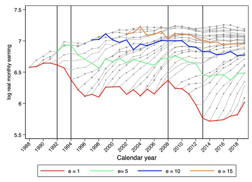
Figure 8 plots the wage profiles, for both monthly earnings and full-time equivalent daily
wages, of new entrants to the labor market with university studies with college and
graduate degrees. Apart from the decreasing trend in the entry wage (the red line) already
highlighted in Section 2, we observe that wages after 5, 10, and 15 years of potential
experience (the green, blue, and orange lines, respectively) follow a similar pattern to
entry wages. Note that the wage profiles for workers with a graduate degree become flat
after 10 years. To some extent this is due to the fact that the CSWL, which is a data set
extracted from social security contribution records, only reports capped earnings when
the cap for the firm’s contribution is reached. For this reason, in our analysis of scarring
effects in Section 4 we stop at 10 years of potential experience.
The figure shows that the decreases in earnings are much higher in the case of workers
with a graduate degree than for those with a college degree. It also makes it apparent that
earnings losses suffered in recessions are not compensated by higher gains in expansions.
This is strongly suggestive of the presence of scarring effects. Interestingly, the later
13cohorts, i.e., those entering after 2010, seem to have steeper wage profiles, but in their
case the impact of the ongoing Covid-19 crisis remains to be seen.
Fig. 8. Wage profiles of new entrants to the labor market by education
(a) College degree
(b) Graduate degree
Note: The left-column figures represent full-time equivalent log real monthly earnings and the right-column
figures full-time equivalent log real daily wages. The levels of these variables are represented for annual
values of potential experience (e), including lines connecting the values for, respectively, 1 (red), 5 (green),
10 (blue), and 15 years (orange). Source: Continuous Sample of Working Lives, Ministerio de Inclusión,
Seguridad Social y Migraciones.
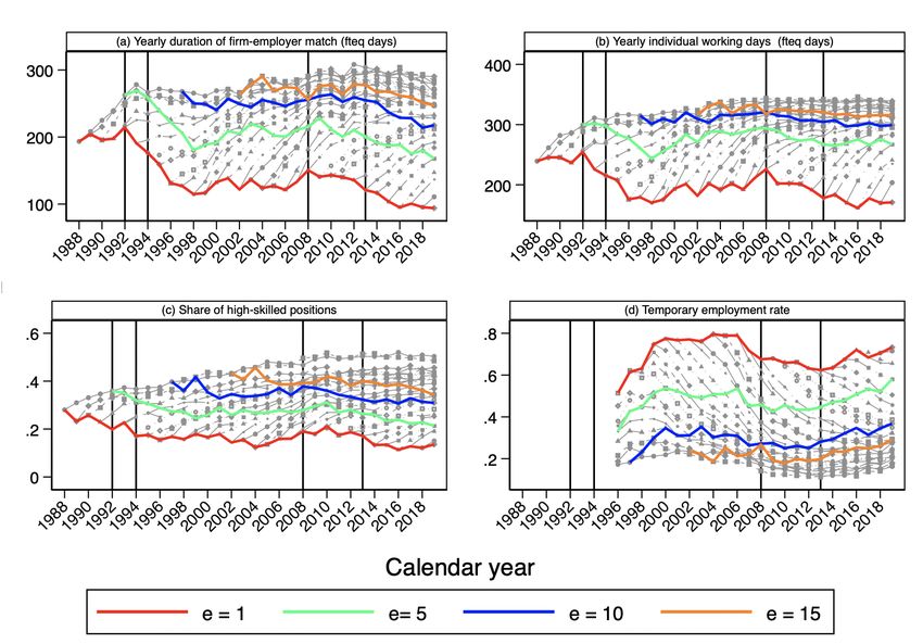
Figure 9 plots the evolution of the share of young workers employed in high skill jobs,
along with annual days worked –both for firm-worker matches and for individual
outcomes–, and the incidence of temporary employment. As in the case of wages, the
initial outcome at the graduation date is highly correlated with the outcomes after 5, 10,
and 15 years of potential experience. In particular, over the sample period, the
deterioration in annual days worked, the lack of gains in the share in high skill jobs, and
the high incidence of temporary employment at graduation are quite persistent. In the next
Section we provide an assessment of the relative importance of scarring effects and a
continuous deterioration of youth labor markets in explaining these patterns.
14Fig. 9. The evolution of the share of high skill jobs, annual days worked and the
share of temporary employment, 1987-2019
Note. The levels of all variables are represented for annual values of potential experience (e), including
lines connecting the values for, respectively, 1 (red), 5 (green), 10 (blue), and 15 years (orange). Temporary
employment data are not representative until 1996. Source: Continuous Sample of Working Lives,
Ministerio de Inclusión, Seguridad Social y Migraciones.
4. Estimating scarring effects and trends in youth employment and earnings
4.1. Empirical strategy
Our empirical strategy for estimating the long-term effects of initial labor market
conditions on youth employment and earnings exploits the variation in unemployment
rates by province of birth and year of graduation but, contrary to the existing literature on
scarring effects (see Oreopoulos et al. 2012, Fernández-Kranz and Rodríguez-Planas
2018), we also allow for a trend component. This component is meant to capture any
systematic changes over time in the earnings-experience profiles of labor market entrants.
As already indicated, our outcomes of interest are the log median real monthly earnings,
log median real daily wage in full-time equivalents, the mean annual days of work in
worker-firm matches, and mean annual days of work per worker, distinguishing between
three education levels (junior college, college, and graduate degrees). We will also present
separate estimations by gender below.
15Let ycpt denote the relevant labor market outcome in period t of a cohort graduated in year
c in province p. We start our exploration with the following cell-level baseline
specification or Model 1, that is estimated for each level of university education:
!!"# = α + β$ γ$ '!"% + θ" + γ$ + )!"# (1)
where qp and ge represent unrestricted province and years of potential experience fixed
effects, respectively, and Ucp0 is the initial province-level unemployment rate at
graduation. Notice that we use the overall unemployment rate at the province level and
not the youth unemployment rate as the latter variable may be affected by changes in the
supply of university graduates. There are 50 provinces, and the sample period is 1987-
2019. Only the first ten years of each cohort, when available, are included in the sample.9
In this specification the be coefficients capture the persistent effects of the initial
conditions at graduation on the labor market outcomes which are allowed to vary with
potential experience. We include fixed effects for a maximum of ten years of potential
experience. Given the presence of experience and province fixed effects, the coefficients
of the interaction term measure changes in experience profiles in earnings and
employment resulting from province-level variations in unemployment rates under the
(unrealistic) assumption that all calendar years and cohorts are the same.
The baseline model implies assuming that there are no changes over time in either the
characteristics of the entering cohorts or the conditions of the youth labor market. Thus,
all cohorts are supposed to be the same (there is no unobserved heterogeneity) and the
labor market outcomes of young workers are assumed to be affected only by the
unemployment rate in the province at which they enter the labor market. In subsequent
steps, we add covariates to the model in order to obtain more reliable estimates of the
scarring effects of the initial conditions once we take into account structural trends,
cohort-specific features, and the persistence in unemployment rates. In a second
specification (Model 2), we add interactions between a linear time trend and the dummies
for years of potential experience. A negative coefficient on these interactions between
trends and experience terms would indicate that youth labor market conditions have
worsened over time due to structural changes in either the demand of labor, the supply of
labor, or the institutional configuration of the labor market. The interactions terms allow
these changes to be different at each year of experience.
Over the more than thirty-year horizon in our sample there are many factors that may
cause these structural shifts in experience profiles. On the supply side, Spain has
witnessed an enormous rise in enrolment in university education, especially among
women. As a consequence, the average quality of university graduates may have changed
over time, while the growth in demand for university graduates lagged behind the growth
in supply in many fields, creating excess supply in the labor market. Moreover, the
introduction of the so-called Bologna process, which created the European Higher
Education Area, shortened the duration of most college degrees from five to four years
and led to a proliferation of new college and graduate degrees. Similarly, on the demand
side, skill-biased technological change may have improved the labor market position of
9
Our sample is a random extraction from the population of Spanish workers. However, since we construct
our sample backwards from the last year (2019), older cohorts are observed for longer lengths of time in
the labor market, which imparts a systematic source of cell-size variation.
16university graduates, but the increased complexity of jobs may also have lengthened their
school-to-work transitions. Last but not least, institutional factors play a key role in
shaping the profiles of entrants. Not only did Spain witness several labor market reforms
(in 1994, 1997, 2006, 2010, 2011, and 2012), but these reforms were often implemented
in the aftermath of recessions and involved measures that relaxed the conditions for the
use of temporary contracts. In other words, the adverse conditions during a recession may
cause structural shifts in entrant profiles due to the endogenous adoption of reforms.
In a final specification (Model 3), to control for unobserved changes in the supply side,
we add unrestricted cohort-specific fixed effects to the set of covariates. These fixed
effects capture all time-invariant cohort-specific features. We also include the
contemporaneous national unemployment rate, which controls for the state of the business
cycle in subsequent years. Oreopoulos et al. (2012) interact this variable with the potential
years of experience fixed effects in order to eliminate lasting effects from the persistence
of unemployment rates. By contrast, here we only filter out the common or average
contemporaneous impact of the unemployment rate on the labor market outcomes of all
cohorts.
4.2 Identification
Our identification procedure relies on the assumption that the year of graduation and the
province of residence are exogenous variables. Selective graduation decisions and self-
selection into migration to other provinces (or countries) would undermine our
identification. However, notice that we use imputed rather than actual graduation ages.
This proxy is exogenous from the perspective of an individual and the same is true of our
proxy for the province of residence. The province of birth is a powerful predictor of the
province of residence at graduation, as almost 90% of Spaniards attend university in their
province of birth.10 For university graduates in the age group below 35 years old, the share
of individuals who live in their province of birth is lower than for university students. To
avoid potential bias in our estimates due to post-graduation migration, as already
indicated, we consider a robustness check in which we collapse the individual-level data
at the level of cohort, province of first employment after graduation, and calendar year.
The results confirm the robustness of our results. Nonetheless, we do not claim that our
estimation captures the causal effect of entering the labor market in a recession on the
long-term outcomes of young workers. Our method is more akin to a decomposition
exercise. Nevertheless, in our choice of specification we have tried to deal with potential
endogeneity issues, that we now discuss.
4.3 Data description
The sample period is 1987-2019 for college and graduate workers. For junior college
workers it is 1987-2013, since these degrees disappeared after 2013 as a result of the
Bologna process. As to other variables, the average national unemployment rate is 17%,
with a standard deviation of 5.3%, ranging from 8.2% to 26.1%. Provincial
unemployment rates show a standard deviation of 7.7%, ranging from 3% to 43.2% The
large variation over time and across provinces helps identify the parameters of interest.
10
Also, the share of people aged 25-34 years old with university degrees who reside in their province of
birth averages 80% for the period 1992-2020 according to the LFS.
17Table 1 presents a set of descriptive statistics at the level of the cells and separately by
education level. All variables except for real monthly earnings are measured in full time
equivalents. See Appendix 1 for details about the construction of our sample.
The Table shows that both earnings and days of work increase with education, as
expected, though the slope between junior college and college is not very pronounced
(with an increase of 17% in monthly earnings). The level of monthly earnings is quite
low, showing extremely low values at the first decile and also low values at the ninth
decile, though they are not adjusted for days or hours of work. Annual days of work by
match are also very low, with the averages going from 5.6 to 7.2 months, which reflects
the prevalence of very short temporary contracts. Annual days by worker are also
relatively low, ranging from 7.5 to 9.2 months per year. The difference between the two
variables indicates that young workers quickly move from one temporary contract to
another.
Table 1. Descriptive statistics of the cohort-province-year cells
Mean Std. dev. P10 P90
Junior College
Real monthly earnings 587.4 217.9 320.2 871.6
Real daily wage 25.8 7.4 18.4 34.1
Annual days worked by match 170.0 68.0 83.2 255.3
Annual days worked by worker 228.4 71.5 130.2 311.3
College
Real monthly earnings 687.8 257.4 345.2 1031.0
Real daily wage 29.2 8.0 19.9 38.7
Annual days worked by match 184.5 64.3 99.4 261.7
Annual days worked by worker 246.1 65.3 154.1 318.6
Graduate
Real monthly earnings 984.1 355.3 486.9 1381.6
Real daily wage 40.7 35.1 25.0 49.3
Annual days worked by match 219.3 80.5 121.9 365.0
Annual days worked by worker 279.8 74.2 190.4 365.0
Note. Period: 1987-2019. The cell sizes are 8,809 for Junior college, 9,929 for College and 7134 for
Graduate degree. The unit of analysis is the cohort-province-year cell. P10 denotes the first decile and P90
the ninth decile. All variables except for real monthly earnings are measured in full time equivalents.
Monthly earnings and wages are expressed in real euros with 1987 as the base year. Source: Continuous
Sample of Working Lives, Ministerio de Inclusión, Seguridad Social y Migraciones.
4.4. Results
Table 2 reports the main results from the estimation of our baseline specification, equation
(1), which includes province and years of potential experience fixed effects, as well as
interactions of the latter with the initial province-level unemployment rate at graduation,
which capture the scarring effects. Table 3 presents the estimates of the specification that
18adds to the baseline the interaction of the potential experience fixed effects with a time
trend. Tables 2 and 3 present only the estimated effects on entry (labeled year 0) and in
the fifth (year 4) and tenth year (year 9), while the full results are included in the online
Appendix.
Table 2. Model 1 estimates of scarring effects
Log real monthly earnings Log real daily wages
Junior Junior
College Graduate College Graduate
college college
U0 x (e=0) .003 -.010*** -.025*** .002 -.004*** -.014***
(.002) (.002) (.003) (.001) (.001) (.002)
U0 x (e=4) -.001 -.012*** -.022*** -.001 -.005*** -.012***
(.001) (.001) (.002) (.001) (.001) (.001)
U0 x (e=9) .005*** .001 -.007*** .001 0.000 -.004***
(.001) (.001) (.002) (.001) (.001) (.001)
Constant 5.902*** 6.037*** 6.786*** 3.098*** 3.183*** 3.605***
(.050) (.047) (.087) (.024) (.020) (.052)
8809 9929 7134 8808 9929 7132
Observations
R-squared 0.535 0.689 0.457 0.52 0.716 0.444
Annual days worked by match Annual days worked by worker
Junior Junior
College Graduate College Graduate
college college
U0 x (e=0) 1.996*** -.020 -2.550*** 1.251*** -.647*** -2.679***
(.288) (.207) (.314) (.314) (.207) (.275)
U0 x (e=4) -.124 -1.824*** -3.558*** -.461** -1.240*** -2.316***
(.216) (.163) (.257) (.195) (.140) (.208)
U0 x (e=9) .572*** -.100 -1.819*** .724*** .406*** -.373
(.193) (.182) (.442) (.156) (.131) (.335)
Constant 71.138*** 82.539*** 205.413*** 127.772*** 150.286*** 282.182***
(8.216) (6.803) (11.329) (8.288) (6.048) (11.334)
8809 9929 7134 8809 9929 7134
Observations
R-squared .524 .662 .377 .636 .764 .399
Note. The model includes fixed effects for the province of birth and years elapsed since graduation.
Standard errors are in parentheses. *** pTable 3. Model 2 estimates of scarring and trend effects
Log real monthly earnings Log real daily wages
Junior Junior
College Graduate College Graduate
college college
U0 x (e=0) -.005** -.007*** -.010*** .002 -.003*** -.006***
(.002) (.001) (.002) (.001) (.001) (.001)
U0 x (e=4) -.008*** -.009*** -.012*** -.002*** -.004*** -.006***
(.001) (.001) (.001) (.001) (.001) (.001)
U0 x (e=9) -.004*** -.004*** -.006*** -.002** -.003*** -.003***
(.001) (.001) (.002) (.001) (.001) (.001)
Trend x (e=0) -.024*** -.0230*** -.048*** .004*** -.007*** -.027***
(.002) (.001) (.002) (.001) (.001) (.002)
Trend x (e=4) -.017*** -.013*** -.022*** -.004*** -.006*** -.013***
(.001) (.001) (.001) (.001) (.001) (.001)
Trend x (e=9) -.016*** -.013*** -.012*** -.007*** -.008*** -.005***
(.001) (.001) (.001) (.001) (.001) (.001)
Constant 6.361*** 6.444*** 7.725*** 3.037*** 3.301*** 4.143***
(.061) (.043) (.078) (.034) (.023) (.047)
Observations 8809 9929 7134 8808 9929 7132
R-squared .641 .799 .655 .538 .755 .625
Annual days worked by match Annual days worked by worker
Junior Junior
College Graduate College Graduate
college college
U0 x (e=0) .628** .416** -.940*** .223 -.288 -1.393***
(.267) (.185) (.238) (.307) (.21) (.237)
U0 x (e=4) -1.143*** -1.496*** -1.947*** -1.089*** -1.150*** -1.291***
(.208) (.184) (.213) (.188) (.163) (.199)
U0 x (e=9) -.96*** -.841*** -1.865*** -.171 .107 -.417
(.195) (.183) (.322) (.18) (.149) (.272)
Trend x (e=0) -4.196*** -3.044*** -4.924*** -3.464*** -2.332*** -4.135***
(.372) (.157) (.29) (.364) (.164) (.25)
Trend x (e=4) -2.557*** -1.939*** -3.863*** -1.549*** -.534*** -2.446***
(.213) (.177) (.253) (.182) (.143) (.219)
Trend x (e=9) -2.7*** -1.861*** -3.118*** -1.515*** -.768*** -2.139***
(.223) (.184) (.335) (.182) (.133) (.29)
Constant 152.74*** 136.86*** 303.72*** 194.13*** 191.51*** 364.10***
(11.699) (6.908) (10.41) (11.236) (6.638) (10.799)
Observations 8809 9929 7134 8809 9929 7134
R-squared .634 .755 .545 .682 .785 .509
Note. The sample period is 1987-2019 for college and graduate degrees. For junior college workers it is
1987-2013. The model includes fixed effects for the province of birth and years elapsed since graduation.
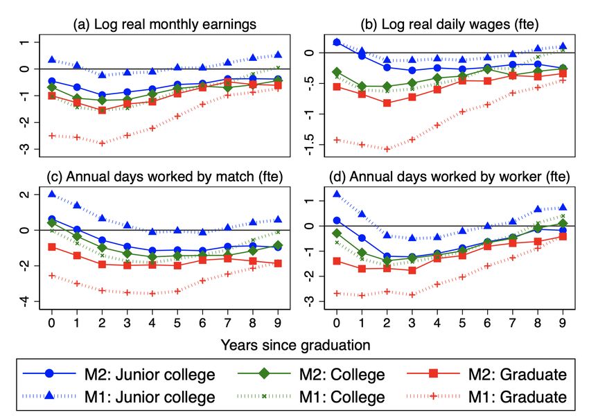
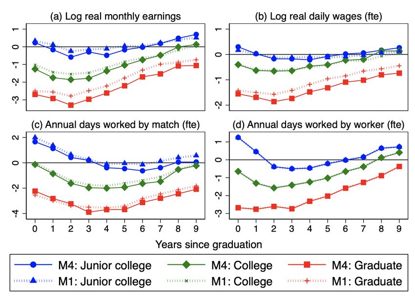
Standard errors are in parentheses. *** pWe discuss the estimated scarring effects using graphs that include the full set of
coefficients. Figure 10 plots the estimated coefficients of the baseline specification or
Model 1 (dashed lines) and the specification with the time trend interactions with
experience or Model 2 (solid lines). Since we have three education groups, four outcome
variables, and several empirical specifications, we will focus on the estimates for college
graduates, who are by far the largest group. The results for the other two education levels
are qualitatively similar, so we will briefly comment on them as we go along.
The estimated coefficients for the baseline Model 1 plotted in Figure 10 clearly suggest
that the initial conditions faced at graduation have a strong and persistent impact on
entrant earnings. For instance, for monthly earnings, the semi-elasticity of with respect to
the unemployment rate at the time of graduation reaches a maximum of -1.5 in the second
year and it becomes -0.5 seven years after graduation, losing significance thereafter. The
coefficients in the graph are multiplied by 100, so this estimate means that an increase of
1 pp in the provincial unemployment rate is associated with a drop in monthly earnings
of 1.5%. To get a sense of magnitudes, this implies that over the Great Recession, a young
person entering the labor market in 2013 in the province with the lowest unemployment
rate in 2007 (Guipúzcoa) would have 13.5% lower monthly earnings two years later than
an entrant in 2007, while the corresponding figure for the province with the largest
unemployment rate (Jaén) would be a staggering 39.4% loss. The impact of
unemployment on the full-time equivalent daily wage in this specification is lower,
reaching a maximum of -0.5 in year 2 and dropping to -0.3 in year 9, which reveals that
part of the effect on monthly earnings comes from lower hours of work.
These estimates are smaller than those for the annual earnings of college graduates in the
related literature.11 In particular, for the US Oreopoulos et al. (2012, Table 2) estimate the
peak effect is -1.8% in years 0-1, even though their specification includes fixed effects
by region of residence, graduation cohort, potential labor market experience, and calendar
year. For Spain, Fernández-Kranz and Rodríguez-Planas (2017, Table 2) estimate a peak
effect of -1.6% in the year of entry, including the same fixed effects as Oreopoulos et al.
(2012) except that they replace the experience fixed effects by a linear and a quadratic
trend.
According to the estimates shown in Figure 10, the impact of 1 pp increase in the
provincial unemployment rate on annual days worked by worker in year 2 is equal to 1.6
days less and to 1.4 less days worked by match (climbing to 1.8 days in year 4).
As Figure 10 makes clear, the estimated scarring effects are significantly lower in Model
2, which includes the interacted linear trends to control for changes in the conditions of
youth labor markets, than in the baseline. The semi-elasticity of monthly earnings to
initial unemployment attains a maximum of -1.2 in year 2 and it is equal to -0.5 for daily
earnings. Similarly, the impact on annual days worked by worker in year 2 is reduced to
1.4 days less and to 1 day on annual days by worker. These effects have a relatively small
magnitude. Thus, while scarring effects are often mentioned as the main culprits of the
worsening of the labor market outcomes of young Spaniards, these results suggest that
there are also other causes of the deterioration of youth wages and employment beyond
the state of the labor market at the time of graduation. And this is in spite of there being
two deep recessions in our sample period (1992-94 and 2008-2013).
11
Note, however, that while these two references estimate the effects on annual earnings, we examine
monthly earnings defined as explained above and in detail in Appendix 1.
21También puede leer